Part 2: Turning 7.7 Million LiDAR Points into a Lightweight 3D Terrain for a Fabric Digital Twin

We turned 7.7 million open LiDAR points into a 6,500-vertex terrain mesh that runs smoothly in any browser by using only free Finnish government data.

In the first part of this blog series we got the Rayfin app scaffolded and deployed to Fabric with a rudimentary 3D model and some procedurally generated terrain. In this post we’ll dig deeper into how we used real laser-scanned terrain data in combination with vector map data to build the realistic terrain model, as well as how Blender was used to generate the wind turbine model.

How to model the terrain accurately?

Our hypothetical wind farm is located in Sievi, Finland, as this area has many wind farms. So we wanted accurate terrain data from the area to support our visualization.

To get good terrain data we went on a hunt for free, open vector map sources. A vector map is a digital map built out of points, lines and polygons rather than pixels, so it can be scaled infinitely without losing sharpness. The National Land Survey of Finland (Maanmittauslaitos) publishes open vector maps that can be used under the CC-BY 4.0 license. You would think this would be a perfect data source for the job? We downloaded the vector map that includes height contours for the area.

The vector map is in the format of an ESRI Shapefile, and we used Python to read the contours from the height layer and turn them into a 3D visualization:

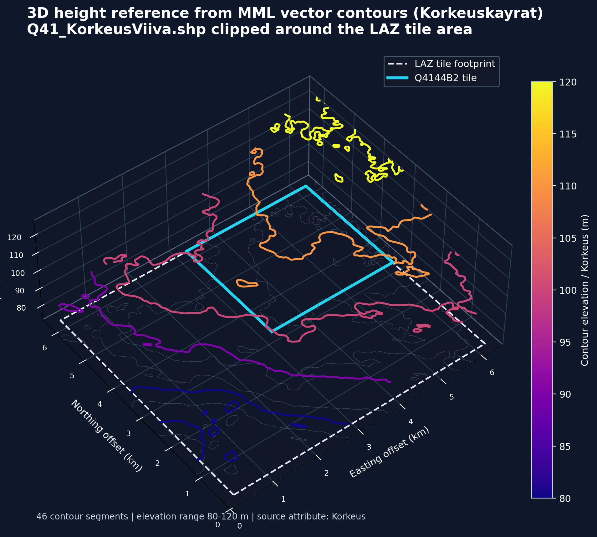
In this image you can see that the wind farm area highlighted in light blue has some elevation detail visible in the vector map data. But the contours turned out to be too sparse to build a convincing surface. For realistic terrain we needed something with much higher resolution. Luckily Maanmittauslaitos also provides laser-scanned (LiDAR) terrain data with a density of 0.5 points per square meter. For the area highlighted in light blue, this means over 7 million points instead of a couple of contour lines.

But this also presents us with a challenge. Visualizing that many points in the browser in real time would be really resource intensive, and we would have far more resolution than we actually need. In the image below you can see the point cloud visualized on a color elevation map. You can notice how detailed it is compared to the vector map.

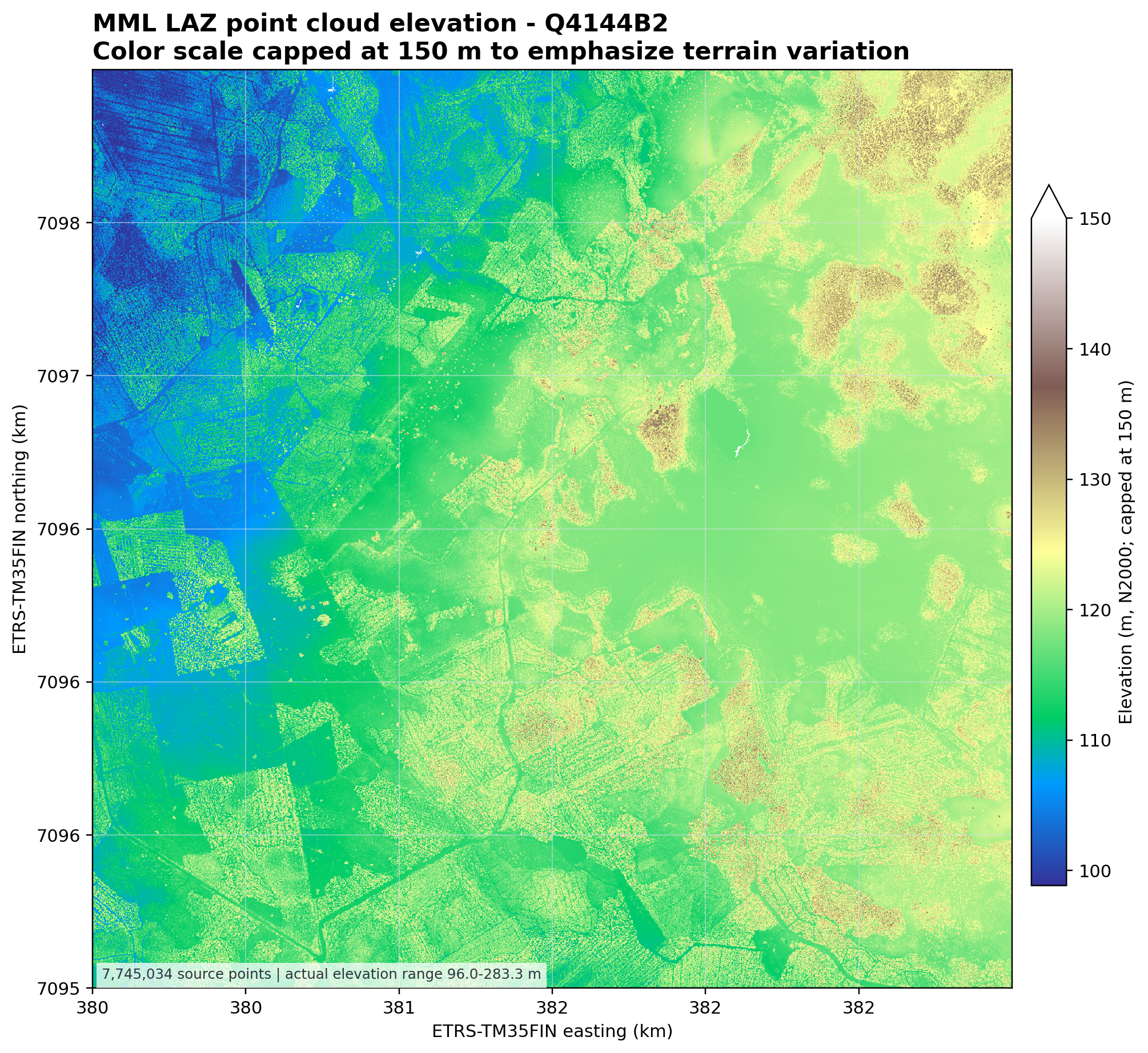
The original laser scanning data was delivered as LAZ point cloud files from Maanmittauslaitos. A LAZ file is a compressed LiDAR point cloud: instead of containing a ready-made surface, it contains millions of individual measurement points. Each point has a real-world coordinate and height value with metadata attached.

For our digital twin, this source data was too detailed to load directly into the browser. A single LAZ tile can contain millions of points, and rendering that raw point cloud in Three.js would be unnecessarily heavy for an interactive web application. Instead, we used the LAZ data as a high-quality source for generating a lighter terrain representation.

The processing step converts the point cloud into a browser-friendly height model. Conceptually, the workflow looks like this:

1. Read the LAZ tile.
2. Extract the point coordinates: easting, northing, and elevation.
3. Crop the data to the area needed by the digital twin.
4. Aggregate the points into a regular height grid.
5. Convert the real-world coordinates into local Three.js coordinates.
6. Build a Three.js terrain mesh from the height grid.
7. Color and light the mesh so terrain shape is visible.

A simplified version of the code looks like this:

import json
import numpy as np
import laspy

LAZ_FILE = "mml/Q4144B2.laz"
OUT_FILE = "public/terrain/q4144b2-heightgrid.json"

GRID_SIZE = 81  # 80 x 80 mesh segments -> 81 x 81 vertices

las = laspy.read(LAZ_FILE)

x = np.asarray(las.x)
y = np.asarray(las.y)
z = np.asarray(las.z)

origin_x = float(x.min())
origin_y = float(y.min())

# Build a regular grid from the point cloud
x_edges = np.linspace(x.min(), x.max(), GRID_SIZE + 1)
y_edges = np.linspace(y.min(), y.max(), GRID_SIZE + 1)

sum_z, _, _ = np.histogram2d(x, y, bins=[x_edges, y_edges], weights=z)
count, _, _ = np.histogram2d(x, y, bins=[x_edges, y_edges])

height = np.divide(
    sum_z,
    count,
    out=np.full_like(sum_z, np.nan, dtype=float),
    where=count > 0,
)

# Fill empty cells with the average height
mean_height = float(np.nanmean(height))
height = np.nan_to_num(height, nan=mean_height)

data = {
    "origin": {
        "easting": origin_x,
        "northing": origin_y,
        "height": float(z.min()),
    },
    "bounds": {
        "minEasting": float(x.min()),
        "maxEasting": float(x.max()),
        "minNorthing": float(y.min()),
        "maxNorthing": float(y.max()),
        "minHeight": float(z.min()),
        "maxHeight": float(z.max()),
    },
    "gridSize": GRID_SIZE,
    "heights": height.tolist(),
}

with open(OUT_FILE, "w") as f:
    json.dump(data, f)

print(f"Wrote {OUT_FILE}")

The final mesh is much lighter than the original point cloud: over 7.7 million source points reduced to roughly 6,500 vertices and 12,800 triangles (an 80×80 segment plane). That makes it suitable for an interactive browser-based digital twin, where we also need to render turbines, labels, weather effects, camera controls, and live operational data.

We also used the vector map data to enrich the terrain with recognizable real-world features. While the LAZ point cloud gives us elevation, the vector layers describe what is on the terrain: roads, rivers, buildings, powerlines, fields, water areas, protected areas, and other map features. These layers can be processed separately and then placed on top of the Three.js terrain mesh.

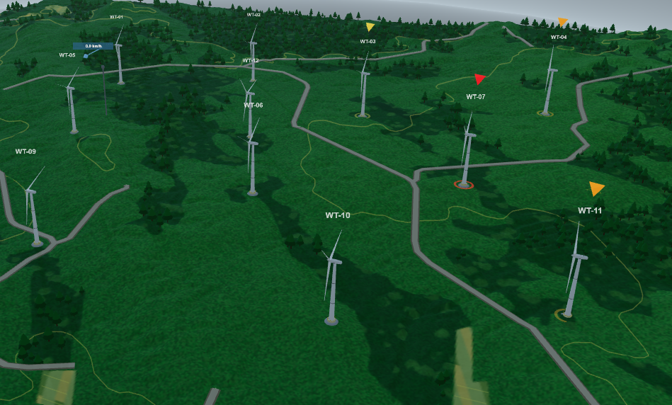
And for the cherry on top, we can add some procedurally generated trees, field terrain and coloring to make the visualization come to life.

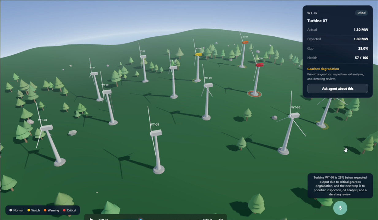
to this:

This lets the digital twin combine two complementary datasets: LAZ provides the shape of the ground, while the vector map layers provide semantic context about what exists on that ground. In some details this is starting to sound like a data processing workflow. And basically it is. We have a huge amount of raw data, and we are refining it to build the end-user presentation. The raw LiDAR data is bronze, the height grid is silver, the rendered scene is the gold layer.

Modeling the wind turbine in Blender

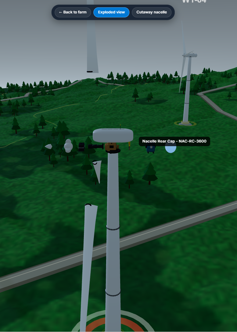
In the first version, a wind turbine could technically be represented with simple geometry. But to support our digital twin use cases we needed the turbine to be more than just a box with a couple of rotating sticks. For a digital twin, visual credibility matters. Users need to immediately understand what they are looking at, trust the scene, and connect the 3D view to the real physical asset. A realistic turbine model makes the environment feel like an operational wind farm rather than a placeholder simulation.

The more accurate model also gives us better interaction points. We can highlight the nacelle, tower, blades, hub, foundation, and other components separately. That matters when the twin is connected to telemetry data, alerts, inspections, and AI explanations. Instead of saying “this box has a warning,” the application can point to the actual turbine component that needs attention.

Realistic geometry also carries the story faster than abstract shapes. Stakeholders do not need to imagine what the asset represents, they can see it. So the goal was not just prettier graphics.

But there was a problem: we didn’t know how to create a realistic 3D model of a wind turbine, and procedural generation would only get us so far. We also couldn’t find any free, open-source models to use in this demo, so we needed to make one ourselves. I first tried generating the turbine procedurally in Three.js with GitHub Copilot, but hit a wall. So I switched approaches: instead of building geometry in the browser, I used Copilot to write a Blender Python script that generates the model as a GLB asset.

To move beyond placeholder geometry, I used GitHub Copilot to help generate a real wind turbine model as a GLB/GLTF asset. Instead of manually modeling the turbine in Blender, I described the structure needed — tower, nacelle, hub, rotor, and blades — and used a Python script to create the geometry procedurally inside Blender.

Blender’s Python API is well suited for this kind of task. The script can create meshes, cylinders, cones, curves, materials, object names, hierarchy, scale, and export settings. That meant I could generate a repeatable turbine asset rather than hand-editing every part. I was pleasantly surprised how well Opus 4.7 was able to create the Blender script.

The generated model included the main turbine components as separate named objects. That was important because the Three.js application does not only display the turbine as a static object. It also needs to interact with parts of it: rotate the rotor, highlight components, apply risk colors, support inspection views, and use raycasting for hover and selection.

The workflow was roughly:

1. Use Copilot to draft a Blender Python script.
2. Run the script to generate the turbine geometry.
3. Create separate objects for the tower, nacelle, rotor, hub, and blades.
4. Assign basic materials and realistic proportions.
5. Name key objects clearly, for example rotor, so Three.js can find them later.
6. Export the result as a compact .glb file.
7. Load the exported model in Three.js with GLTFLoader.

In the app, the final asset is loaded from:

/models/wind-turbine.glb

Three.js loads it once as a prototype, then clones it for each turbine in the wind farm. This keeps the application efficient while still giving each turbine its own state, material changes, highlighting, and animation.

Conclusion

In my mind this was probably the most satisfying part of this whole demo-building exercise. We saw how the open LiDAR data turned into a terrain mesh that represents real terrain, and how the turbine got a real bill of materials with realistic parts, visuals and telemetry.

In the next part we will wire this whole thing together: connecting the digital twin to a Foundry Agent that provides a chat and voice experience.

← Back home